Overview
The PROTEX model is a time-variant, process-based (mechanistic), integrative model that supports describing the entire journey of chemicals from production to dose in the human body. PROTEX allows you to assess ecological and human exposures based on information on chemical, population, and the regional environment.
PROTEX contains four modules, which can be run either separately or jointly:
The rationale and technical details of PROTEX can be found in Li et al. 2018a and Li et al. 2018b. Note that PROTEX has been updated substantially since its first publication. Descriptions in earlier publications may sometimes differ from what is described here.
PROTEX contains four modules, which can be run either separately or jointly:
- An technosphere module, based on substance flow analysis theory, simulates the time-variant accumulation, flows, and multimedia emissions of a chemical during industrial processes, indoor and outdoor use phases (“in-use stocks”), and end-of-life disposal (“waste stock”) of consumer articles, i.e., the human socioeconomic system. (From production to emissions)
- A regional fate and transport module, based on the fugacity approach, simulates time-variant chemical concentrations in different environmental media (e.g., air, water, soil, sediment, vegetation, artificial surfaces, etc.) of nested indoor-urban-rural environments. (From emissions to environmental concentrations)
- A food-web bioaccumulation module, based on the fugacity approach, simulates the accumulation of a chemical in aquatic and terrestrial organisms from the ambient environment and food items, as well as resulting concentrations in their tissues. These organisms eventually become foodstuff in our dinning tables. (From environmental concentrations to food concentrations)
- A human exposure and toxicokinetic module, based on the fugacity approach, simulates time-variant human exposure to the chemical via multiple exposure routes from near- and far-field environments, as well as resulting concentrations in the body. (From environmental and food concentrations to human exposure)
The rationale and technical details of PROTEX can be found in Li et al. 2018a and Li et al. 2018b. Note that PROTEX has been updated substantially since its first publication. Descriptions in earlier publications may sometimes differ from what is described here.
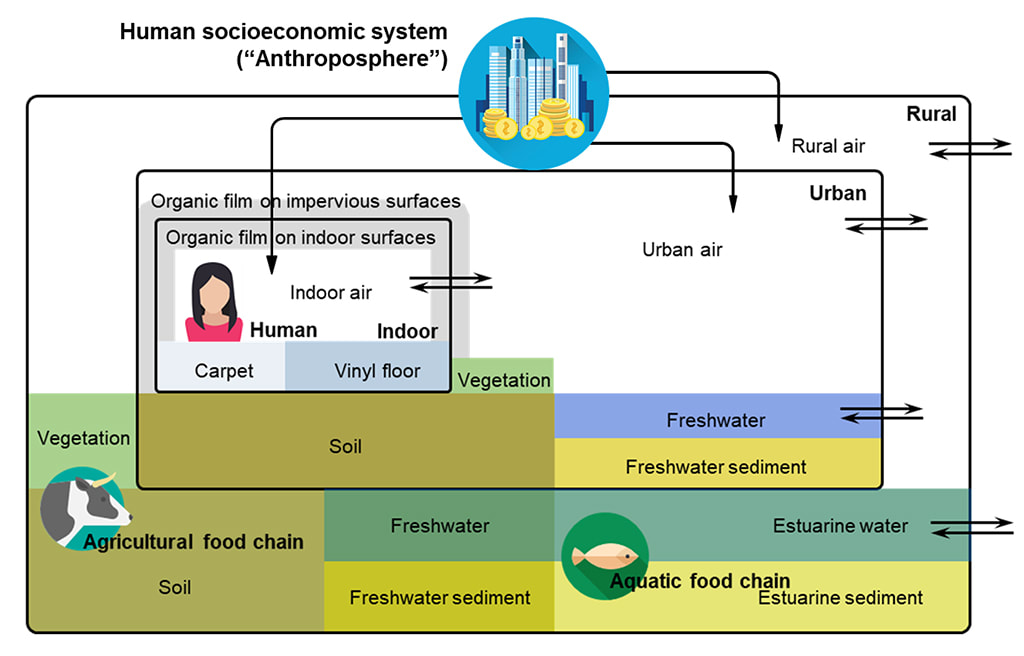
The structure of PROTEX
|
A quick start
Here is a hands-on tutorial to walk you through features and functions in PROTEX and to illustrate how to calculate the life-course exposure of an archetypal female Canadian, who was born in 1950 and lives in the city, to a chemical called BDE-47, as presented in Li et al. 2020.
First, let us navigate to the “Start” page.
On this page you are able to select data from built-in databases for a rapid run.
1. Select the scenario of modeling from built-in databases: the chemical, population, and the regional environment that you want to simulate for. In this illustrative case, you need to select “BDE-47” from the drop-down list of chemicals, “Canadian (Average)” from the drop-down list of populations, and “Canada-side Lake Ontario drainage basin” from the drop-down list of regional environments. Once you are done with the selection of an item, do not forget to click the “select” button: this will load all data to corresponding spreadsheets in PROTEX so that you will not be bothered to enter data individually.
The "Start" page
2. Specify the timeframe of modeling: The start and end years of your simulation. In most cases, the start year of simulation is the first year that the chemical of interest is produced or consumed in the region. In this illustrative case, we enter 1970 as the start year and 2030 as the end year according to the years mentioned in Li et al. 2020.
3. Specify the birth year of the modeled individual: The year that the target individual is born. In this illustrative case, we enter 1950 as the birth year.
4. Control output options: You can determine whether you want the model to show some intermediate parameters. Outputting all intermediate parameters sometimes takes a long time.
5. Specify exposure routes: For each exposure route, you can enter a decimal between 0 and 1 to indicate the extent to which you weigh this exposure route. For instance, you can enter “1” if you want to take full consideration of an exposure route, “0” if you want to exclude an exposure route from your modeling, or “0.5” if you think the modeled individual is exposed to only half of the potential dose (e.g., the modeled individual wears a face mask, which reduces inhalation exposure by half). In this illustrative case, we enter 1 for all exposure routes.
Next, let us navigate to the “Input_technosphere” sheet.
On this page, you need to enter information on chemical production and use.
1. Enter tonnage information such as annual tonnage (total production or consumption) in metric ton, fraction used in the region, fraction used indoors, and fraction entering regional waste stock, expected lifespans for indoor and outdoor uses, for each year in the modeled timeframe. You can enter information for at most 200 years, if desired.
- Tips: You can find lifespans of most commodities via the Lifespan database for Vehicles, Equipment, and Structures (LiVES).
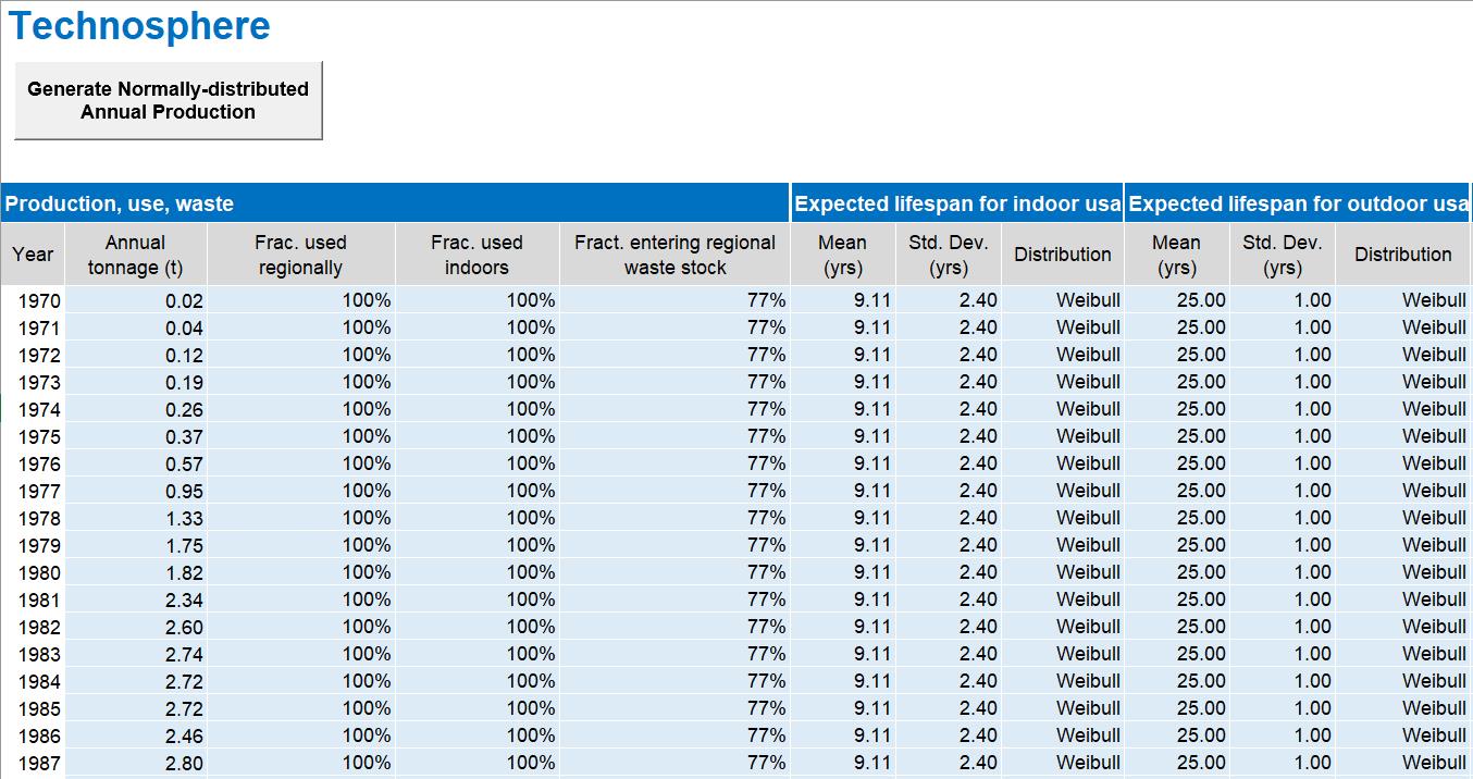
The "Input_technosphere" page
|
2. Enter emission factors associated with industrial processes, indoor use, outdoor use, and waste disposal. Emission factors should be decimals between 0 and 1. You can enter either time-variant (i.e., to specify emission factors for individual years) or time-independent emission factors (i.e., to apply the same emission factors to all years in the modeled timeframe) to PROTEX. When you enter both, the time-variant emission factors are given the priority in PROTEX modeling. Please do not forget to specify environmental compartments receiving emissions no matter entering time-variant or time-independent emission factors. In this illustrative case, we enter the numbers shown in Li et al. 2020.
- Tips: You may find emission factors for industrial processes from Specific Environmental Release Categories (spERC), US EPA's AP-42 emission factors compilation, or the EU's Technical Guidance Documents. You may also calculate emission factors associated with chemical use using computational tools.
- If the data on hand are annual emission rates rather than annual tonnage, you can skip the technosphere calculation by entering these annual emission rates directly to the "annual tonnage (t)" column and using an emission factor of 1 to the receiving compartment of interest.
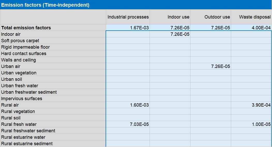
The "Input_technosphere" page
|
Next, let us navigate to the “Input_Human” sheet.
You can see that information on the general Canadian population (e.g., activity and lifestyle) has been loaded when you clicked “Select” button in the “Start” sheet. Now you need to specify the modeled individual is a female, lives in the urban area, and consumes groundwater as drinking water.
You can see that information on the general Canadian population (e.g., activity and lifestyle) has been loaded when you clicked “Select” button in the “Start” sheet. Now you need to specify the modeled individual is a female, lives in the urban area, and consumes groundwater as drinking water.
Part of the "Input_human" page
|
The final step is to navigate back to the “Start” sheet.
If you want to run PROTEX for all results from production to exposure, please click “Complete calculation”.
If you want partial results, you may run one or more modules individually. For instance, you may click “1. Technosphere” if you want PROTEX to output emission estimates only. You may click “1. Technosphere”, “2. Environment”, and “3. Food webs” if you want PROTEX to assess ecological exposures. Alternatively, you may click “1. Technosphere”, “2. Environment”, “3. Food webs”, and “4.2 Within-age trend” if you want PROTEX to depict the within-age trend of chemical concentrations in the human body.
To run the PROTEX model
Advanced modeling
The above case illustrates how to perform PROTEX modeling using the combination of chemical, population, and regional environment already in PROTEX databases. Of course, this may not be your case. If the chemical, population, or the regional environment is not there, you can enter the information directly to PROTEX.
Input chemical information
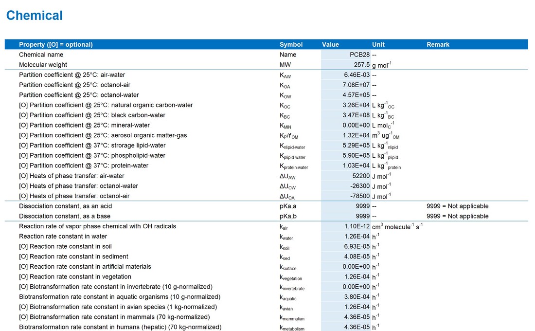
Please navigate to “Input_chemical” sheet. On this page, you can enter the properties of the modeled chemical, including
1. Chemical name: mandatory
2. Molecular weight: mandatory
3. Two of the three standard equilibrium partition coefficients KOW, KOA, and KAW: mandatory
For optional parameters with default values available in PROTEX, you can always overwrite the numbers if you disagree with PROTEX.
Input chemical information
Please navigate to “Input_chemical” sheet. On this page, you can enter the properties of the modeled chemical, including
1. Chemical name: mandatory
2. Molecular weight: mandatory
3. Two of the three standard equilibrium partition coefficients KOW, KOA, and KAW: mandatory
- Tips: The high quality of input data is the key to the success of modeling. It is recommended to give values adjusted for “thermodynamically internal consistency” the highest priority because they are believed to be the most reliable. If these values are not available, you can let PROTEX compute automatically the partition coefficients using the ppLFER approach: please leave these partition coefficients blank and enter the ppLFER descriptors (see the instruction below). You can also enter partition coefficients sourced from experimental databases, handbooks, or computational tools such as ACD-Labs, OPERA and EPI Suite.
- Tips: PROTEX computes these values using the ppLFER approach if ppLFER descriptors are entered (see the instruction below), or using Trouton’s Rule if otherwise.
- Tips: Please enter pKa if the modeled chemical is an acid or (14 - pKb) if the modeled chemical is a base. The value can be computed using computational tools such as ACD-Labs and OPERA. Please leave it blank or enter 9999 if the modeled chemical does not dissociate in the environment.
- Tips: Experimental or observational value is preferred. It can also be computed by prediction models such as Arnot et al. 2014 or Papa et al. 2014. This parameter is not required if you assess ecological exposures only.
- You do not need to enter a value here if you have the data of "human hepatic intrinsic clearance" (see below). However, if you enter both, this human intrinsic biotransformation rate constant will be given the higher priority in PROTEX modeling.
- Tips: Experimental or observational value is preferred. It can also be computed by computational tools such as OPERA and EPI Suite.
- Tips: If not entered, the reaction rate constant in vegetation is assumed to be equal to that in water; the reaction rate constant in soil is assumed to be half that in water; the reaction rate constant in sediment is assumed to be 1/10 that in water (for more information for these empirical relationships, please see Fenner et al. 2005). Other extrapolation factors, e.g., 1:1:1/4 (Boethling et al. 1995) and 1:1/2:1/9 (Aronson et al. 2006), have also been published for converting water rate constants to soil and sediment rate constants. If hydrolysis and photolysis are negligible, then the reaction rate constant in water can be approximated by the biodegradation rate constant, which can be computed using Arnot et al. 2005 (preferred) or OPERA (preferred for hydrocarbons).
- Reaction rate constant in artificial surfaces is not required if you assess ecological exposures or human exposure from far-field environments.
- Tips: Experimental or observational values are preferred. They can also be calculated by prediction models, e.g., by Brown et al. 2012, Papa et al. 2014, and OPERA for biotransformation rate constants in fish, and by Papa et al. 2018 and Arnot et al.2014 for biotransformation rate constants in humans. If not entered, the biotransformation rate constant in birds is extrapolated from that in mammals using an allometric relationship in PROTEX.
- These biotransformation rate constants are not required if you assess human exposure from near-field environments only (e.g., in the case of indoor exposure to disinfecting chemicals).
- Tips: If not entered, built-in default values are used by PROTEX.
- Tips: In order to enable PROTEX to automatically compute partition coefficients and heats, you need to find these pp-LFER descriptors from the UFZ-LSER database. These pp-LFER descriptors are not required if you do not intend to have PROTEX perform pp-LFER calculations.
- Tips: The value can be computed by prediction tools such as OPERA. If not entered, it is assumed to be 100% (the most conservative value).
- Tips: This parameter is required only when the human intrinsic biotransformation rate constant is not entered (see above).
For optional parameters with default values available in PROTEX, you can always overwrite the numbers if you disagree with PROTEX.
The "Input_chemical" page
|
Input human information
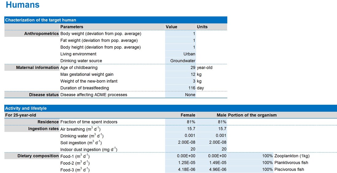
Please navigate to the “Input_human” sheet. On this page, you can enter information on the population to which the modeled individual belongs, as well as the specific information about the modeled individual, including
1. Demographic feature of the modeled individual: Biological sex (female and male), living environment (urban or rural), and drinking water source (surface or ground water).
2. Maternal information if you run PROTEX for a woman: Age of childbearing, maximum gestational weight gain during the pregnancy, the weight of the new-born infant, and the duration of breastfeeding.
- Tips: If you do not know this maternal information, you can just proceed with the defaults in PROTEX.
- These parameters are not required if you run PROTEX for a man.
Part of the "Input_human" page
|
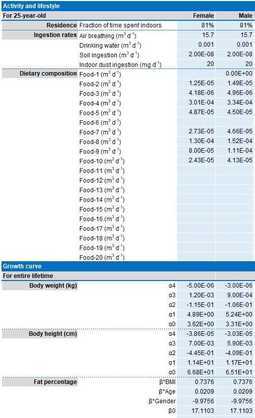
3. Activity and lifestyle of a 25-year-old individual: Fraction of time spent indoors, rates of ingestion of exposure media (air, drinking water, soil particles, and indoor dust), and dietary composition
- Tips: These data can be found mostly from Exposure Factors Handbooks developed by environmental or health authorities in your country (e.g., here is an example by the U.S. Environmental Protection Agency). PROTEX automatically extrapolates these data to other ages using built-in empirical equations.
- PROTEX allows users to define up to 20 plants or animal-based food items (10 already defined in PROTEX, including leafy vegetables, root plant, beef, milk, chicken, and pork). To define a plant or an animal, you just need to enter information to the "DB_foodweb" sheet ("DB" means "database"), including the living environment (urban or rural), temperature change (ectotherm or homeotherm), volumetric body composition, food intake preference, rates of ingestion of environmental media (air, water, soil particles), reproductive information, parameters controlling the absorption efficiencies through ingestion and inhalation, and age-dependent growth curve. PROTEX will compute bioaccumulation based on the numbers entered.
Part of the "DB_foodweb" page
|
4. Parameters controlling the growth curve.
- Tips: PROTEX uses quartic functions (polynomials of degree four) to describe the age dependent changes in body weight and height. PROTEX correlates fat percentage with BMI, age, and sex using multivariate relationships. You can find these empirical relationships from medical or health publications. However, you can just proceed with the defaults in PROTEX if you do not have the information.
Input environmental information
Please navigate to the “Input_environment” sheet. On this page, you can find a wide range of parameters characterizing individual compartments of the modeled environment. Please feel free to change overwrite the values of cells in light blue if you would like to, but do not be overwhelmed! You do not have to change every single parameter on this page because (i) certain parameters differ quite little between regions, (ii) modeling results are not quite sensitive to certain parameters, or (iii) accurate site-specific values are not available for certain parameters. It is acceptable and also recommended, to use default generic values for parameters that are largely universal to most regions.
To achieve the best performance of modeling, you are recommended to use region-specific values for parameters that are highly unique to the region of interest, including
1. The total regional area
2. Population in the region
3. Land use information: Urban and rural fractions of the region. For the urban area, the fractions of residential (indoor) area, impervious surfaces (e.g., pavements), vegetation canopy, fresh water, bare soil. For the rural area, the fractions of unforested soils, forest, fresh water, and estuary water. For the indoor area, the fractions of soft and porous carpet, rigid and impermeable flooring, and hard contact surfaces.
4. Meteorology & hydrology information: Atmospheric residence time in the urban and rural environments; air exchange rate between the indoor and urban environments; typical aerosol concentrations in the urban and rural environments; annual precipitation; monthly temperature, wind speed, and hydroxyl radical concentration in the rural environment.
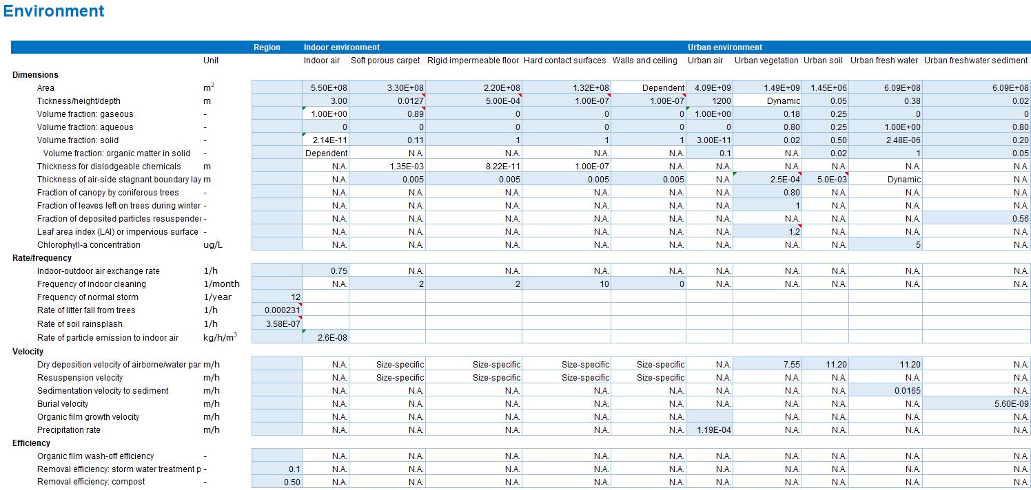
Part of the "Input_environment" page
Download
You can download the latest version of PROTEX (license valid until Jan 01, 2022). Please contact Dr. Li Li if you still want to use the model after the expiration of the license.
